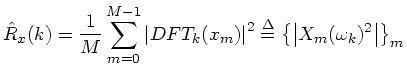
Welch's Method for Power Spectrum Estimation

Welch's method (or the periodogram method) for estimating power spectra [36] is carried out by dividing the time signal into successive blocks, and averaging squared-magnitude DFTs of the signal blocks. Let $x_m$ denote the $m$th block of the signal $x$, and let $M$ denote the number of blocks. Then the PSD estimate is given by

$${\hat R}_x(k) = \frac{1}{M}\sum_{m=0}^{M-1}\left\vert DFT_k(x_m)\... ...t\vert^2 \isdef \left\{\left\vert X_m(\omega_k)^2\right\vert\right\}_m \protect$$ (E.3)

where we have introduced the notation `` $\{\cdot\}_m$'' to denote time averaging across blocks (or ``frames'') of data indexed by $m$.

However, note that $\left\vert X_m\right\vert^2\leftrightarrow x\star x$ which is circular autocorrelation. To avoid this, we use zero padding in the time domain, i.e., we replace $x_m$ above by $[x_m,0,\ldots,0]$. However, note that although the ``wrap-around problem'' is fixed, the estimator is still biased. That is, its expected value is the true autocorrelation $r_x(l)$ weighted by $N-\vert l\vert$. This bias is equivalent to having multiplied the correlation in the ``lag domain'' by a triangular window (also called a ``Bartlett window''). The bias can be removed by simply dividing it out, as in Eq. (E.2). However, it is common to retain this inherent Bartlett weighting since it merely corresponds to smoothing the power spectrum (or cross-spectrum) with a sinc$^2$ kernel; it also down-weights the less reliable large-lag estimates, weighting each lag by the number of lagged products that were summed.

For real signals, the autocorrelation is real and even, and therefore the power spectral density is real and even for all real signals. The PSD $R_x(\omega)$ can interpreted as a measure of the relative probability that the signal contains energy at frequency $\omega$. Essentially, however, it is the long-term average energy density vs. frequency in the random process $x(n)$.

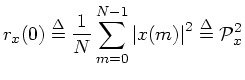
At lag zero, the autocorrelation function reduces to the average power (root mean square) which we defined earlier:

$$r_x(0) \isdef \frac{1}{N}\sum_{m=0}^{N-1}\left\vert x(m)\right\vert^2 \isdef {\cal P}_x^2$$

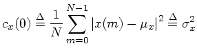
Replacing ``correlation'' with ``covariance'' in the above definitions gives the corresponding zero-mean versions. For example, the cross-covariance is defined as

$$\zbox {c_{xy}(n) \isdef \frac{1}{N}\sum_{m=0}^{N-1}\overline{[x(m)-\mu_x]} [y(m+n)-\mu_y]}$$

We also have that $c_x(0)$ equals the variance of the signal $x$:

$$c_x(0) \isdef \frac{1}{N}\sum_{m=0}^{N-1}\left\vert x(m)-\mu_x\right\vert^2 \isdef \sigma_x^2$$