Continuous/Discrete Fourier Transforms
 Welch's Method for Power Spectrum Estimation
 Signal Processing Analysis Contents
Global
Contents
Signal Processing Analysis Contents
Global
Contents
 Global
Index Index Search
Global
Index Index Search
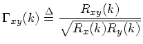
A function related to cross-correlation
is the coherence function  , defined in terms of power
spectral densities and the cross-spectral
density by
, defined in terms of power
spectral densities and the cross-spectral
density by
In practice, these quantities can be estimated by averaging
 ,
,  and
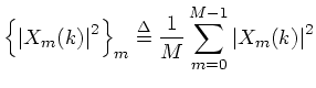
and  over successive signal blocks. Let
 denote time averaging
across frames as in Eq. (E.3)
of §E.3
above Then the time average of , for example, is given by
where
denote time averaging
across frames as in Eq. (E.3)
of §E.3
above Then the time average of , for example, is given by
where  is the DFT of the
  th
block of time data
th
block of time data  , and
, and  is the total
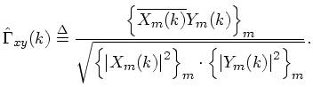
number of time blocks available. In this notation, an estimate of the coherence,
the sample coherence function
is the total
number of time blocks available. In this notation, an estimate of the coherence,
the sample coherence function  , may be defined by
The magnitude-squared coherence
, may be defined by
The magnitude-squared coherence  is a real function between 0 and
 which gives a measure of correlation
between
which gives a measure of correlation
between  and
and  at each frequency
(DFT bin
number
at each frequency
(DFT bin
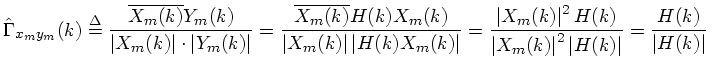
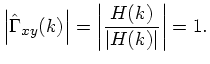
number  ). For example, imagine that is produced from via an LTI
filtering operation:
Then the coherence function in each frame is
and the magnitude-squared coherence function is simply
On the other hand, when and are uncorrelated
(e.g., is a noise process not
derived from ), the coherence converges to zero at
all frequencies.
). For example, imagine that is produced from via an LTI
filtering operation:
Then the coherence function in each frame is
and the magnitude-squared coherence function is simply
On the other hand, when and are uncorrelated
(e.g., is a noise process not
derived from ), the coherence converges to zero at
all frequencies.
A common use for the coherence function is in the validation of input/output
data collected in an acoustics experiment for purposes of system
identification. For example,  might be a known signal which is input to an unknown system, such as a
reverberant room, say, and
might be a known signal which is input to an unknown system, such as a
reverberant room, say, and  is the recorded response of the
room. Ideally, the coherence should be at all frequencies.
However, if the microphone is situated at a null
in the room response for some frequency, it may record mostly noise at that
frequency. This will be indicated in the measured coherence by a significant dip
below .
is the recorded response of the
room. Ideally, the coherence should be at all frequencies.
However, if the microphone is situated at a null
in the room response for some frequency, it may record mostly noise at that
frequency. This will be indicated in the measured coherence by a significant dip
below .
Continuous/Discrete Fourier Transforms
Welch's Method for Power Spectrum Estimation
Signal Processing Analysis Contents
Global
Contents
Global
Index Index Search
``Mathematics of the Discrete
Fourier Transform (DFT)'', by Julius O. Smith III, (online
book).
(Browser settings
for best viewing results)
(How to cite
this work)
(Order a
printed hardcopy)
Copyright © 2003-08-28 by Julius O. Smith III
Center for Computer Research in Music and
Acoustics (CCRMA), Stanford
University
 (automatic links
disclaimer)
(automatic links
disclaimer)